Generalized Pareto Distribution (GPD)
Generalized Pareto Distribution (GPD) is a family of of continuos probability distributions and is often used to model the tails of another distribution. It is sometimes specified by three parameters : location, shape and scale, but it can also be specified by only shape and scale parameters. Visit Wikipedia page for more information.
Functions
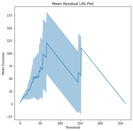
1. MRL(sample, alpha=0.05)
Mean Residual Life plot takes mean of excess values above a threshold minus threshold and plots it against that threshold value. If the plot is linear that is ok but if the plot starts loosing stability then choose that threshold value.
Parameters
sample : pandas dataframe
the whole dataset
alpha : float a number giving 1-alpha confidence levels to use. Default value is 0.05.
Returns
None
Expand for source code
     #Mean Residual Life Plot for finding appropriate threshold value.
     def MRL(sample, alpha=0.05):

    #Defining the threshold array and its step
    step = np.quantile(sample.iloc[:,1], .995)/60
    threshold = np.arange(0, max(sample.iloc[:,1]), step=step)
    z_inverse = stats.norm.ppf(1-(alpha/2))

    #Initialization of arrays
    mrl_array = []
    CImrl = []

    #First Loop for getting the mean residual life for each threshold value and the
    #second one getting the confidence intervals for the plot
    for u in threshold:
        excess = []
        for data in sample.iloc[:,1]:
            if data > u:
                excess.append(data - u)
        mrl_array.append(np.mean(excess)) #
        std_loop = np.std(excess)
        CImrl.append(z_inverse*std_loop/(len(excess)**0.5))

    CI_Low = []
    CI_High = []

    #Loop to add in the confidence interval to the plot arrays
    for i in range(0, len(mrl_array)):
        CI_Low.append(mrl_array[i] - CImrl[i])
        CI_High.append(mrl_array[i] + CImrl[i])

    #Plot MRL
    plt.figure(figsize=(7,7))
    sns.lineplot(x = threshold, y = mrl_array)
    plt.fill_between(threshold, CI_Low, CI_High, alpha = 0.4)
    plt.xlabel('Threshold')
    plt.ylabel('Mean Excesses')
    plt.title('Mean Residual Life Plot')
    plt.show()
Example
#Mean Residual Life plot for finding appropriate threshold
#value for Peak-Over-Threshold method.
ely.MRL(sample=data,alpha=0.05)
Output
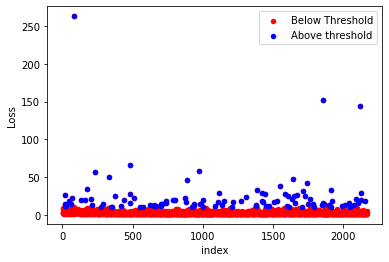
2. getPOT(sample, threshold)
In Peak-Over-Threshold method the values greater than a given threshold are taken as extreme values.
Parameters
sample : pandas dataframe
The whole Dataset
threshold : integer
An integer value above which the values are taken as extreme values.
Returns
exce : pandas dataframe
Excess values obtained.
Expand for source code
      #Peaks-Over-Threshold method for finding large values.
      def getPOT(sample,threshold):
          colnames=list(sample)
          exce=sample[sample.iloc[:,1].gt(threshold)]

          #Plotting the excess values obtained using POT method.
          ax = sample.iloc[:,1].reset_index().plot(kind='scatter', x='index', y=colnames[1],
                                           color='Red', label='Below Threshold')
          exce.reset_index().plot(kind='scatter', x='index', y=colnames[1],
                                          color='Blue', label='Above threshold', ax=ax)
          return exce
Example
#Getting large claims using POT method using threshold value as 30.
pot=ely.getPOT(sample=data,threshold=10)
pot
Output
        Date     Loss
index
15 	1980-01-26 	11.374817
17 	1980-01-28 	26.214641
22 	1980-02-13 	14.122076
24 	1980-02-19 	11.713031
28 	1980-02-23 	12.465593
... 	... 	...
2105 	1990-09-08 	14.851485
2121 	1990-10-08 	144.657591
2122 	1990-10-10 	28.630363
2123 	1990-10-12 	19.265677
2150 	1990-12-10 	17.739274

109 rows × 2 columns
3. gpdfit(sample, threshold)
GPD is a family of continous probability distributions and is often used to model the tails of another distribution. It is specified by two parameters - Shape and scale parameters.
Parameters
sample : pandas dataframe
The whole Dataset
threshold : integer An integer value above which the values are taken as extreme values.
Returns
Estimated distribution parametrs of GPD fit, sample excess values and value above the threshold.
Expand for source code
    #Fit the large claims obtained from POT method to Generalized Pareto distribution (GPD).
    def gpdfit(sample, threshold):
        sample = np.sort(sample.iloc[:,1])
        sample_excess = []
        sample_over_thresh = []
        for data in sample:
            if data > threshold+0.00001:
                sample_excess.append(data - threshold)
                sample_over_thresh.append(data)
        series=pd.Series(sample)
        series.index.name="index"
        dataset = Dataset(series)

        #Using PeaksOverThreshold function from evt library.
        pot = PeaksOverThreshold(dataset, threshold)
        mle = GPDMLE(pot)
        shape_estimate, scale_estimate= mle.estimate()
        shape=getattr(shape_estimate, 'estimate')
        scale=getattr(scale_estimate, 'estimate')
        return(shape, scale,sample, sample_excess, sample_over_thresh,mle)
Example
#Fitting GPD with large claims obtained using POT method.
gpdfit=ely.gpdfit(sample=data,threshold=10)
4. gpdparams(fit)
Getting estimated distribution parameters for GPD fit.
Parameters
fit : object
Object containing information about GPD fit.
Returns
None
Expand for source code
    #Get estimated distribution parameters for GPD fit.
    def gpdparams(fit):
        shape=fit[0]
        scale=fit[1]
        print("Shape:",shape)
        print("Scale:",scale)
Example
#Getting estimated distribution parameters for GPD fit.
ely.gpdparams(fit=gpdfit)
Output
Shape: 0.49697630118112623
Scale: 6.9754506314014675
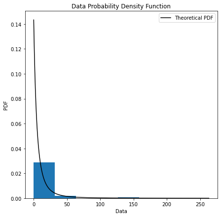
5. gpdpdf(sample, threshold, bin_method, alpha)
Probability density plots are used to understand data distribution for a continuous variable and we want to know the likelihood (or probability) of obtaining a range of values that the continuous variable can assume.
Parameters
sample : pandas dataframe
The whole Dataset
threshold : integer
An integer value above which the values are taken as extreme values.
bin_method : string
Binning algorithm, specified as one of the following - auto, scott, fd, sturges, integers and sqrt.
alpha : float
a number giving 1-alpha confidence levels to use. Default value is 0.05.
Returns
None
Expand for source code
     #get PDF plot with histogram to diagnostic the model
     def gpdpdf(sample, threshold, bin_method, alpha):
         [shape, scale, sample, sample_excess, sample_over_thresh] = gpdfit(sample, threshold)
         x_points = np.arange(0, max(sample), 0.001)
         pdf = stats.genpareto.pdf(x_points, shape, loc=0, scale=scale)

         #Plotting PDF
         plt.figure(figsize=(7,7))
         plt.xlabel('Data')
         plt.ylabel('PDF')
         plt.title('Data Probability Density Function')
         plt.plot(x_points, pdf, color = 'black', label = 'Theoretical PDF')
         plt.hist(sample_excess, bins = bin_method, density = True)
         plt.legend()
         plt.show()
Example
#Data Probability Density Function plot.
ely.gpdpdf(sample=data,threshold=10,bin_method="sturges",alpha=0.05)
Output
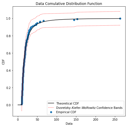
6. gpdcdf(sample, threshold, alpha)
The cumulative distribution function of a real-valued random variable X, or just distribution function of X, evaluated at x, is the probability that X will take a value less than or equal to x.
Parameters
sample : pandas dataframe
The whole Dataset
threshold : integer
An integer value above which the values are taken as extreme values.
alpha : float
a number giving 1-alpha confidence levels to use. Default value is 0.05.
Returns
None
Expand for source code
    #plot gpd cdf with empirical points
    def gpdcdf(sample, threshold, alpha):
        [shape, scale, sample, sample_excess, sample_over_thresh] = gpdfit(sample, threshold)
        n = len(sample_over_thresh)
        y = np.arange(1,n+1)/n

        i_initial = 0
        n = len(sample)
        for i in range(0,n):
            if sample[i] > threshold:
                i_initial = i
                break

        #Computing confidence interval with the Dvoretzky–Kiefer–Wolfowitz method based on the empirical points
        F1 = []
        F2 = []
        for i in range(i_initial,len(sample)):
            e = (((mt.log(2/alpha))/(2*len(sample_over_thresh)))**0.5)
            F1.append(y[i-i_initial] - e)
            F2.append(y[i-i_initial] + e)

         x_points = np.arange(0, max(sample), 0.001)
         cdf = stats.genpareto.cdf(x_points, shape, loc=threshold, scale=scale) #getting theoretical cdf

        #Plotting cdf
        plt.figure(figsize=(7,7))
        plt.plot(x_points, cdf, color = 'black', label='Theoretical CDF')
        plt.xlabel('Data')
        plt.ylabel('CDF')
        plt.title('Data Comulative Distribution Function')
        plt.scatter(sorted(sample_over_thresh), y, label='Empirical CDF')
        plt.plot(sorted(sample_over_thresh), F1, linestyle='--', color='red', alpha = 0.8, lw = 0.9, label = 'Dvoretzky–Kiefer–Wolfowitz Confidence Bands')
        plt.plot(sorted(sample_over_thresh), F2, linestyle='--', color='red', alpha = 0.8, lw = 0.9)
        plt.legend()
        plt.show()
Example
#Cumulative Density Function plot.
ely.gpdcdf(sample=data,threshold=10,alpha=0.05)
Output
7. gpdqqplot(sample,threshold,alpha)
QQplot is a graphical technique for determining if two datasets come from populations with a common distribution. A 45 degree reference line is plotted, if the two sets come from populations with the same distribution, the points should fall approximately along this reference line.
Parameters
sample : pandas dataframe
The whole Dataset
threshold : integer
An integer value above which the values are taken as extreme values.
alpha : float
a number giving 1-alpha confidence levels to use. Default value is 0.05.
Returns
None
Expand for source code
    #Plot QQplot with empirical points.
    def gpdqqplot(sample, threshold, alpha):

        [shape, scale, sample, sample_excess, sample_over_thresh] = gpdfit(sample, threshold) #fit data
        i_initial = 0
        p = []
        n = len(sample)
        sample = np.sort(sample)
        for i in range(0, n):
            if sample[i] > threshold + 0.0001:
                i_initial = i #get the index of the first observation over the threshold
                k = i - 1
                break

        for i in range(i_initial, n):
             p.append((i - 0.35)/(n)) #using the index, compute the empirical probabilities by the Hosking Plotting Poistion Estimator.

        p0 = (k - 0.35)/(n)

        quantiles = []
        for pth in p:
           quantiles.append(threshold + ((scale/shape)*(((1-((pth-p0)/(1-p0)))**-shape) - 1))) #getting theorecial quantiles arrays

        n = len(sample_over_thresh)
        y = np.arange(1,n+1)/n #getting empirical quantiles

        #Kolmogorov-Smirnov Test for getting the confidence interval
        K = (-0.5*mt.log(alpha/2))**0.5
        M = (len(p)**2/(2*len(p)))**0.5
        CI_qq_high = []
        CI_qq_low = []
        for prob in y:
            F1 = prob - K/M
            F2 = prob + K/M
            CI_qq_low.append(threshold + ((scale/shape)*(((1-((F1)/(1)))**-shape) - 1)))
            CI_qq_high.append(threshold + ((scale/shape)*(((1-((F2)/(1)))**-shape) - 1)))

        #Plotting QQ
        plt.figure(figsize=(7,7))
        sns.regplot(quantiles, sample_over_thresh, ci = None, line_kws={'color':'black','label':'Regression Line'})
        plt.axis('square')
        plt.plot(sample_over_thresh, CI_qq_low, linestyle='--', color='red', alpha = 0.5, lw = 0.8, label = 'Kolmogorov-Smirnov Confidence Bands')
        plt.legend()
        plt.plot(sample_over_thresh, CI_qq_high, linestyle='--', color='red', alpha = 0.5, lw = 0.8)
        plt.xlabel('Theoretical GPD Quantiles')
        plt.ylabel('Sample Quantiles')
        plt.title('Q-Q Plot')
        plt.show()
Example
#Quantile-Quantile plot.
ely.gpdqqplot(sample=data,threshold=10,alpha=0.5)
Output

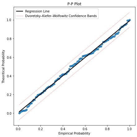
8. gpdppplot(sample, threshold, alpha)
PP-plot is used for assessing how closely two datasets agree. It plots the two cumulative distribution functions against each other.
Parameters
sample : pandas dataframe
The whole Dataset
threshold : integer
An integer value above which the values are taken as extreme values.
alpha : float
a number giving 1-alpha confidence levels to use. Default value is 0.05.
Returns
None
Expand for source code
    #probability-probability plot to diagnostic the model
    def gpdppplot(sample, threshold, alpha):
        [shape, scale, sample, sample_excess, sample_over_thresh] = gpdfit(sample, threshold)
        n = len(sample_over_thresh)
        y = np.arange(1,n+1)/n
        cdf_pp = stats.genpareto.cdf(sample_over_thresh, shape, loc=threshold, scale=scale)

        #Getting Confidence Intervals using the Dvoretzky–Kiefer–Wolfowitz method
        i_initial = 0
        n = len(sample)
        for i in range(0, n):
            if sample[i] > threshold + 0.0001:
                i_initial = i
                break
        F1 = []
        F2 = []
        for i in range(i_initial,n):
            e = (((mt.log(2/alpha))/(2*len(sample_over_thresh)))**0.5)
            F1.append(y[i-i_initial] - e)
            F2.append(y[i-i_initial] + e)

        #Plotting PP
        plt.figure(figsize=(7,7))
        sns.regplot(y, cdf_pp, ci = None, line_kws={'color':'black', 'label':'Regression Line'})
        plt.plot(y, F1, linestyle='--', color='red', alpha = 0.5, lw = 0.8, label = 'Dvoretzky–Kiefer–Wolfowitz Confidence Bands')
        plt.plot(y, F2, linestyle='--', color='red', alpha = 0.5, lw = 0.8)
        plt.legend()
        plt.title('P-P Plot')
        plt.xlabel('Empirical Probability')
        plt.ylabel('Theoritical Probability')
        plt.show()
Example
#Probability-Probaility plot.
ely.gpdppplot(sample=data,threshold=10,alpha=0.5)
Output
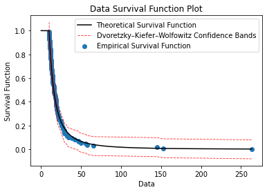
9. survivalFunction(sample, threshold, alpha)
The survival function is a function that gives the probability that the object of interest will survive past a certain time.
Parameters
sample : pandas dataframe
The whole Dataset
threshold : integer
An integer value above which the values are taken as extreme values.
alpha : float
a number giving 1-alpha confidence levels to use. Default value is 0.05.
Returns
None
Expand for source code
    #Plot the survival function, (1 - cdf)
    def survivalFunction(sample, threshold, alpha):
        [shape, scale, sample, sample_excess, sample_over_thresh] = gpdfit(sample, threshold)

        n = len(sample_over_thresh)
        y_surv = 1 - np.arange(1,n+1)/n

        i_initial = 0

        n = len(sample)
        for i in range(0, n):
            if sample[i] > threshold + 0.0001:
                i_initial = i
                break
        #Computing confidence interval with the Dvoretzky–Kiefer–Wolfowitz
        F1 = []
        F2 = []
        for i in range(i_initial,len(sample)):
            e =  (((mt.log(2/alpha))/(2*len(sample_over_thresh)))**0.5)
            F1.append(y_surv[i-i_initial] - e)
            F2.append(y_surv[i-i_initial] + e)

        x_points = np.arange(0, max(sample), 0.001)
        surv_func = 1 - stats.genpareto.cdf(x_points, shape, loc=threshold, scale=scale)

        #Plotting survival function
        plt.figure(9)
        plt.plot(x_points, surv_func, color = 'black', label='Theoretical Survival Function')
        plt.xlabel('Data')
        plt.ylabel('Survival Function')
        plt.title('Data Survival Function Plot')
        plt.scatter(sorted(sample_over_thresh), y_surv, label='Empirical Survival Function')
        plt.plot(sorted(sample_over_thresh), F1, linestyle='--', color='red', alpha = 0.8, lw = 0.9, label = 'Dvoretzky–Kiefer–Wolfowitz Confidence Bands')
        plt.plot(sorted(sample_over_thresh), F2, linestyle='--', color='red', alpha = 0.8, lw = 0.9)
        plt.legend()
        plt.show()
Example
#Survival Function
ely.survivalFunction(sample=data,threshold=10,alpha=0.05)
Output